What does three decades of ocean tides sound like? In this project, I worked with Claude to pull 30 years of water level measurements from a NOAA tide gauge in Boston Harbor and convert them directly into an audio waveform — no synthesis, no simulation, just real data played back as sound.
The result is a 60-second tone that encodes every storm surge, spring tide, and seasonal shift from 1995 to 2025 into something you can hear.
Listen: Boston Harbor, 1995–2025
NOAA Station 8443970 · 6-min water level data sonified at 44.1 kHz
The Data: Where It Comes From
The data comes from NOAA's Center for Operational Oceanographic Products and Services (CO-OPS), specifically their Tides & Currents API. The station is 8443970 — Boston, MA, a well-instrumented, long-running tide gauge located at 42.3539°N, 71.0503°W.
This station records the water level relative to Mean Sea Level (MSL) every 6 minutes, 24 hours a day, and has been doing so since 1995. That's the finest standard interval CO-OPS offers (1-minute data exists but is limited to tiny request windows).
The Pull
The API allows a maximum of one month per request, so fetching 30 years required 372 sequential API calls, each requesting a one-month window:
STATION_ID = "8443970"  # Boston, MA
PRODUCT    = "water_level"
DATUM      = "MSL"  # Mean Sea Level
UNITS      = "metric"
INTERVAL   = "6"  # 6-minute intervals

START_DATE = datetime(1995, 1, 1)
END_DATE   = datetime(2025, 12, 31, 23, 59)
The monthly windows are generated and iterated through one at a time, with a polite 1-second delay between requests:
def generate_monthly_windows(start: datetime, end: datetime):
    """Yield (begin, end) pairs, each spanning up to one calendar month."""
    current = start
    while current < end:
        next_month = (current.replace(day=1) + timedelta(days=32)).replace(day=1)
        window_end = min(next_month - timedelta(minutes=1), end)
        yield current, window_end
        current = next_month
Each window hits the CO-OPS REST API and returns JSON with timestamped water level readings. Failed requests are retried up to 3 times with exponential backoff:
def fetch_window(begin: datetime, end: datetime, retries: int = 3):
    """Fetch a single month window with retries."""
    url = build_url(begin, end)
    for attempt in range(1, retries + 1):
        try:
            with urlopen(url, timeout=30) as resp:
                data = json.loads(resp.read().decode())
            if "error" in data:
                return []
            return data.get("data", [])
        except (URLError, HTTPError, json.JSONDecodeError) as e:
            if attempt < retries:
                time.sleep(2 * attempt)
    return []
What We Got
The full pull took about 17 minutes and produced a 113 MB CSV:
| Metric | Value |
|---|---|
| Total records | 2,676,106 |
| Valid values | 2,665,469 |
| Missing / bad | 10,637 |
| Min water level | −2.550 m |
| Max water level | +3.037 m |
| Range | 5.587 m |
| Mean | +0.082 m (above MSL) |
Visualizing the Waves
Before turning the data into sound, it helps to see what we're working with.
Full 30-Year Time Series
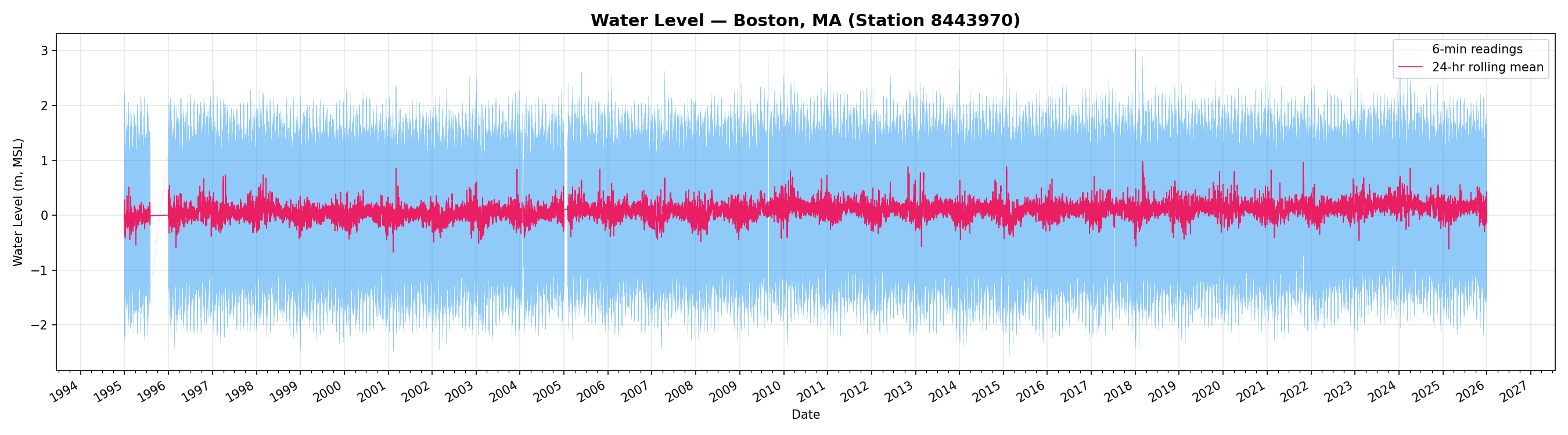
The blue trace shows the raw 6-minute readings — the characteristic saw-tooth pattern of semi-diurnal tides. The pink overlay is a 24-hour rolling mean, which smooths out the tidal oscillation and reveals seasonal variation and longer-term trends. Occasional spikes from storm surges (nor'easters and hurricanes) are clearly visible as sharp excursions.
7-Day Zoom: Individual Tidal Cycles
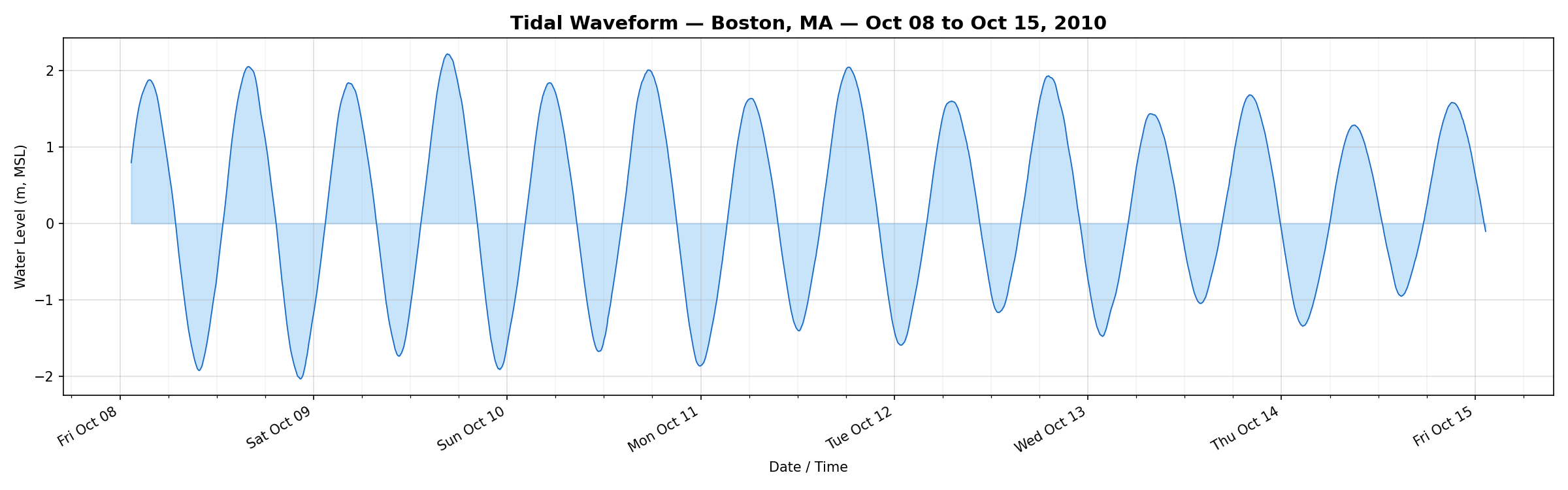
Zooming into a single week, the semi-diurnal pattern is unmistakable: roughly two high tides and two low tides per day. Boston's tidal range here is about 3–4 meters — among the larger ranges on the U.S. East Coast.
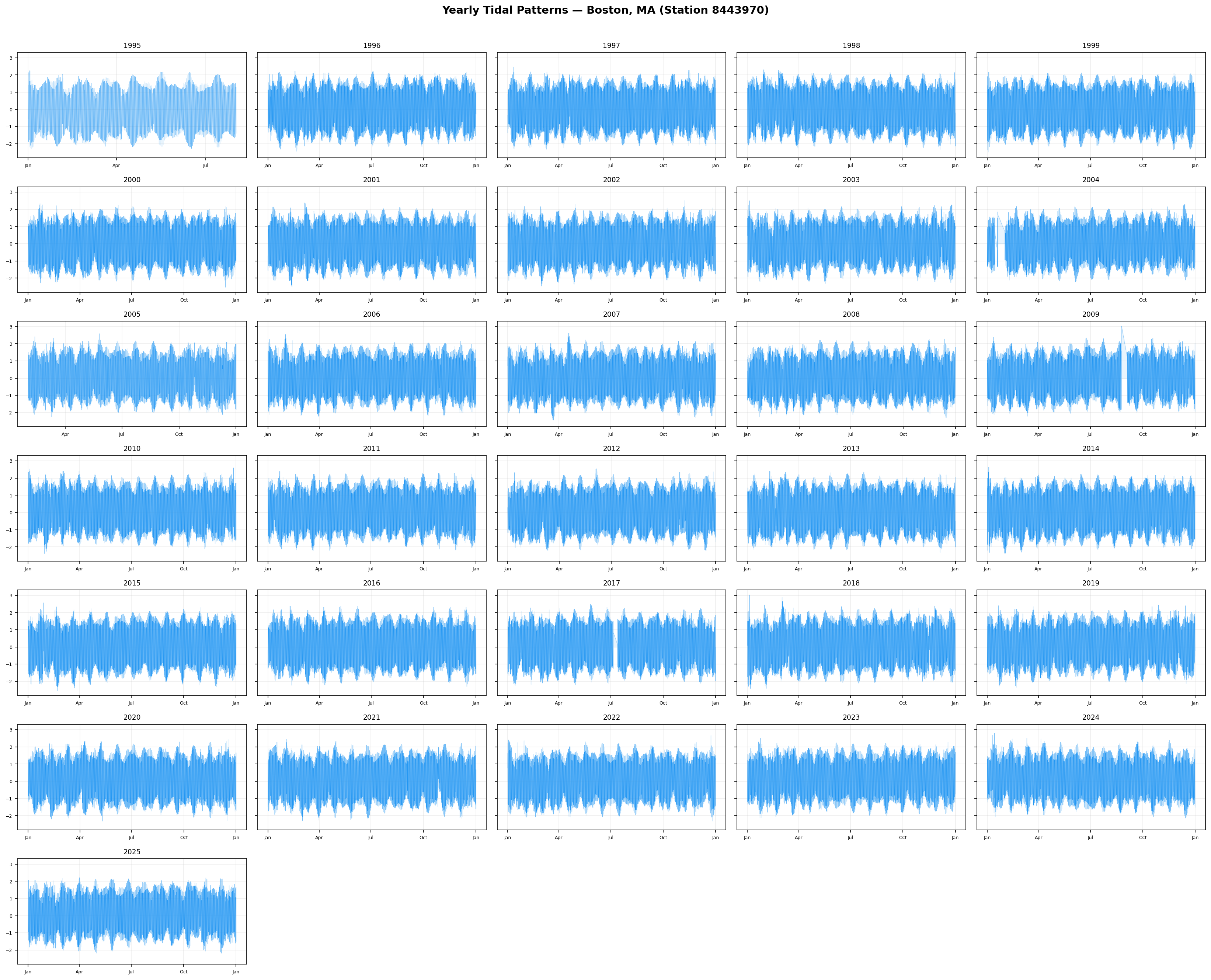
Year-by-Year Comparison
Spectral Analysis: The Frequencies Hidden in the Data
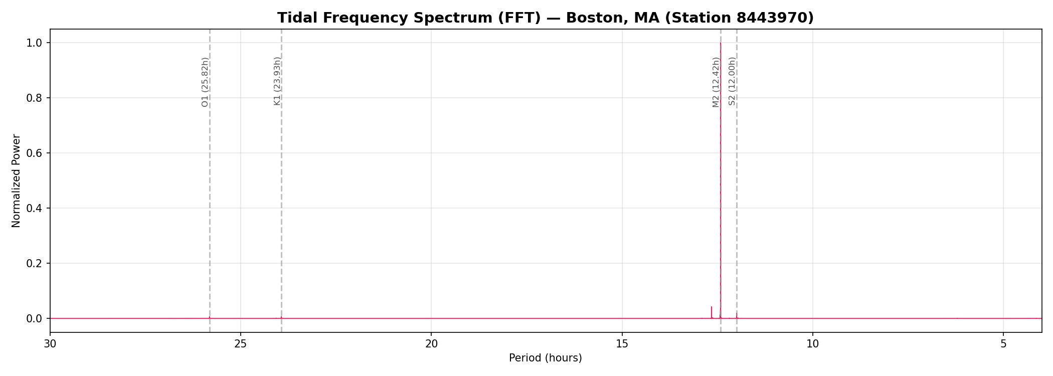
An FFT of the full dataset reveals the dominant frequencies in the signal. The overwhelming peak is at M2 (12.42 hours) — the principal lunar semi-diurnal constituent. This is the Moon's gravitational pull creating two tidal bulges as the Earth rotates. The nearby S2 (12.00 hours) is the solar semi-diurnal tide. Further out, K1 (23.93h) and O1 (25.82h) represent diurnal constituents.
This spectrum is the key to understanding why the audio sounds the way it does.
The Transformation: Data to Audio
The core idea is simple and direct: treat each water level measurement as a single audio sample. No filtering, no pitch-shifting, no effects — just the raw data, normalized and written into a WAV file.
Step 1: Load and Clean
The CSV values are loaded and any gaps (about 10,600 out of 2.67 million — less than 0.4%) are filled with linear interpolation:
def load_values():
    """Load water level values from CSV."""
    values = []
    with open(CSV_FILE, newline="") as f:
        for row in csv.DictReader(f):
            try:
                values.append(float(row["v"]))
            except (ValueError, KeyError):
                values.append(float("nan"))
    return np.array(values)


def interpolate_nans(arr):
    """Linear interpolation over NaN gaps."""
    nans = np.isnan(arr)
    if not nans.any():
        return arr
    x = np.arange(len(arr))
    arr[nans] = np.interp(x[nans], x[~nans], arr[~nans])
    return arr
Step 2: Normalize to Audio Range
Audio samples need to be in the [−1, 1] range. The normalization maps the full tidal range (from −2.55 m to +3.04 m) linearly onto this interval:
def normalize(arr):
    """Normalize to [-1, 1] range."""
    mn, mx = arr.min(), arr.max()
    return 2.0 * (arr - mn) / (mx - mn) - 1.0
A water level of −2.55 m becomes −1.0 and +3.04 m becomes +1.0. Every intermediate value maps proportionally.
Step 3: Write the WAV File
The normalized samples are written as a 16-bit mono WAV at 44,100 Hz — standard CD-quality sample rate. The file is built from scratch with no audio libraries, just struct and NumPy:
def write_wav(filename, samples, sample_rate):
    """Write 16-bit mono WAV file."""
    n = len(samples)
    clipped = np.clip(samples, -1.0, 1.0)
    pcm = (clipped * 32767).astype(np.int16)

    with open(filename, "wb") as f:
        # RIFF header
        data_size = n * 2  # 16-bit = 2 bytes per sample
        f.write(b"RIFF")
        f.write(struct.pack("<I", 36 + data_size))
        f.write(b"WAVE")
        # fmt chunk
        f.write(b"fmt ")
        f.write(struct.pack("<IHHIIHH", 16, 1, 1, sample_rate,
                            sample_rate * 2, 2, 16))
        # data chunk
        f.write(b"data")
        f.write(struct.pack("<I", data_size))
        f.write(pcm.tobytes())
The RIFF/WAVE header is constructed byte by byte: format tag (PCM = 1), one channel, 44,100 Hz sample rate, 16 bits per sample.
The Math of the Mapping
Here's where it gets interesting. The ~2,676,000 samples played at 44,100 Hz produce about 60.7 seconds of audio. The time compression ratio is enormous:
- 30 years of real time → 60 seconds of audio
- 1 second of audio ≈ 6 months of ocean data
The semi-diurnal tidal cycle has a real-world period of 12.42 hours. At 6-minute sampling, that's about 124 samples per cycle. When those 124 samples are played back at 44,100 Hz, the resulting frequency is:
44100 Hz / 124 samples ≈ 355 HzStep 4: Waveform Display Data
For the web player above, the full 2.67 million samples are downsampled to 4,000 display points using min-max bucketing — each bucket preserves both extremes so the visual waveform retains its shape:
def downsample_for_display(arr, n_points):
    """Min-max downsampling: for each bucket, keep both min and max."""
    bucket_size = len(arr) // n_points
    result = []
    for i in range(n_points):
        chunk = arr[i * bucket_size : (i + 1) * bucket_size]
        result.append({"min": float(chunk.min()), "max": float(chunk.max())})
    return result
What You Hear
The audio is a sustained tone centered around 355 Hz with rich texture. What you're hearing isn't synthesized — it's the actual shape of tidal oscillations played back as a pressure wave through your speakers. Variations in the sound encode real phenomena:
- The base pitch (~355 Hz) — The Moon's semi-diurnal gravitational pull
- Subtle beating / pulsing — Interference between lunar and solar tides (spring/neap cycle)
- Amplitude swells — Seasonal tidal variation and storm surges
- Gradual pitch / texture drift — Long-term changes in tidal patterns and sea level
Use the player above to explore — slow down to examine individual events or speed up to hear longer patterns compressed further.
Tools Used
- Data source — NOAA CO-OPS Tides & Currents API
- Language — Python 3 (NumPy, Matplotlib)
- Audio — Raw PCM WAV generation with
struct, no audio libraries - Visualization — Matplotlib with Agg backend
- Player — Vanilla HTML/JS with Web Audio API and Canvas
The entire pipeline — from API fetch to playable audio — runs with just Python and NumPy.